Modelling the unimproved value in the ACT's Woden Valley

Goal

The goal of this case study is to show how to use allhomes to pull in past sales data for various ACT suburbs and then fit a mixed-effect model using Stan to predict the unimproved value (UV, i.e. the value of the plot of land itself) as a function of the block size (in square-meters), the year of the sale and the suburb. We then explore the output of the model and interpret its results.

Taking inspiration from examples & modelling discussions given in Gelman, Hill and Vehtari, Regression and Other Stories, this case study also serves as an example of how to fit a mixed-effect model to real-world data and interpret results; as will become clear, the model fit is not particularly good in the sense that a lot of the observed variability remains unexplained by the model’s input variables. However, the case study is useful in the context of exploring model results and different aspects of the model fit, and represents the kind of analysis one might perform when exploring a new real-world dataset.

Prerequisities

We load necessary non-base R libraries, optimise the use of multiple cores for running the rstanarm model, and define a colour palette based on the nice wesanderson package.

library(allhomes)
library(tidyverse)
library(rstanarm)
library(bayesplot)
library(tidybayes)
library(modelr)
library(wesanderson)
library(plotly)
options(mc.cores = parallel::detectCores())
pal <- wes_palette("GrandBudapest1", n = 3)

Raw data

We get past sales for all suburbs in ACT’s Woden Valley from the last 10 years. This is easily done by using the allhomes::divisions_ACT dataset, and then filter divisions (i.e. suburbs) based on their corresponding SA3 regions.

suburbs <- divisions_ACT |>
        filter(sa3_name_2016 == "Woden Valley") |>
        unite(suburb, division, state, sep = ", ") |>
        pull(suburb)
data <- suburbs |> 
    map_dfr(function(burb) 
        map_dfr(2011L:2020L, function(yr) get_past_sales_data(burb, yr)))
#> Warning in get_past_sales_data(burb, yr): No sales data for suburb 'O'Malley,
#> ACT'
#> Warning in get_past_sales_data(burb, yr): No sales data for suburb 'O'Malley,
#> ACT'
#> Warning in get_past_sales_data(burb, yr): No sales data for suburb 'O'Malley,
#> ACT'
#> Warning in get_past_sales_data(burb, yr): No sales data for suburb 'O'Malley,
#> ACT'
#> Warning in get_past_sales_data(burb, yr): No sales data for suburb 'O'Malley,
#> ACT'
#> Warning in get_past_sales_data(burb, yr): No sales data for suburb 'O'Malley,
#> ACT'
#> Warning in get_past_sales_data(burb, yr): No sales data for suburb 'O'Malley,
#> ACT'
#> Warning in get_past_sales_data(burb, yr): No sales data for suburb 'O'Malley,
#> ACT'
#> Warning in get_past_sales_data(burb, yr): No sales data for suburb 'O'Malley,
#> ACT'
#> Warning in get_past_sales_data(burb, yr): No sales data for suburb 'O'Malley,
#> ACT'
#> Warning in get_past_sales_data(burb, yr): No sales data for suburb 'Swinger
#> Hill, ACT'
#> Warning in get_past_sales_data(burb, yr): No sales data for suburb 'Swinger
#> Hill, ACT'
#> Warning in get_past_sales_data(burb, yr): No sales data for suburb 'Swinger
#> Hill, ACT'
#> Warning in get_past_sales_data(burb, yr): No sales data for suburb 'Swinger
#> Hill, ACT'
#> Warning in get_past_sales_data(burb, yr): No sales data for suburb 'Swinger
#> Hill, ACT'
#> Warning in get_past_sales_data(burb, yr): No sales data for suburb 'Swinger
#> Hill, ACT'
#> Warning in get_past_sales_data(burb, yr): No sales data for suburb 'Swinger
#> Hill, ACT'
#> Warning in get_past_sales_data(burb, yr): No sales data for suburb 'Swinger
#> Hill, ACT'
#> Warning in get_past_sales_data(burb, yr): No sales data for suburb 'Swinger
#> Hill, ACT'
#> Warning in get_past_sales_data(burb, yr): No sales data for suburb 'Swinger
#> Hill, ACT'

Data processing

Since we want to build a predictive model that allows us to estimate the residential unimproved value (UV) of a property based on its block size and location, we keep only those records where we have data for the UV and block size (i.e. we omit records where any of these fields are NA) and further limit block sizes to less than 2000 sqm and UVs to less than 2 million dollars (this is to exclude large commercial purchases).

data_model <- data |>
    mutate(year = as.integer(year(contract_date))) |>
    select(division, unimproved_value, block_size, year) |>
    filter(
        if_all(everything(), ~ !is.na(.x) & .x > 0),
        block_size < 2000, unimproved_value < 2e6) %>%
    # Variable transformations
    mutate(
        # Year since 2019
        year_since = year - 2019L,
        # log-transformed UV
        log_UV = log(unimproved_value),
        # log-transformed block_size, standardised to the log of median value
        log_block_size_std = log(block_size) - log(850))
data_model
#> # A tibble: 3,439 × 7
#>    division unimproved_value block_size  year year_since log_UV
#>    <chr>               <int>      <int> <int>      <int>  <dbl>
#>  1 Chifley            360000        853  2011         -8   12.8
#>  2 Chifley            444000       1048  2011         -8   13.0
#>  3 Chifley            359000        695  2011         -8   12.8
#>  4 Chifley            341000        822  2011         -8   12.7
#>  5 Chifley            451000        760  2011         -8   13.0
#>  6 Chifley            410000        845  2011         -8   12.9
#>  7 Chifley            450000       1330  2011         -8   13.0
#>  8 Chifley            382000        857  2011         -8   12.9
#>  9 Chifley            366000       1020  2011         -8   12.8
#> 10 Chifley            486000        990  2011         -8   13.1
#> # ℹ 3,429 more rows
#> # ℹ 1 more variable: log_block_size_std <dbl>

Fitting the model

Model formulation

We now use rstanarm to fit a model using full Bayesian inference in Stan. We assume that the effects that the log-transformed block size and the (shifted) year have on the log-transformed UV vary by division (i.e. suburb). To model this, we consider a fixed and a random effect component to both the overall intercept and predictor coefficient estimates: The fixed effects characterise the effects that are common across divisions, and the random effects are expressed as deviations from the fixed effects that vary across divisions.

Written out, the model takes the following form

$\begin{align} \mathtt{log\_UV} &\sim N\left(\mu, \sigma\right)\\ \mu &= \mu_\alpha + \alpha_{[i]} + \left(\mu_{\beta_1} + \beta_{1, [i]} \right) \mathtt{year\_since} + \left(\mu_{\beta_2} + \beta_{2,[i]}\right) \mathtt{log\_block\_size\_std}\\ \end{align}$

where $\begin{align} \mathtt{year\_since} &= \mathtt{year} - 2019\,,\\ \mathtt{log\_block\_size\_std} &= \log{(\mathtt{block\_size})} - \log{(850)}\,. \end{align}$ Such a model is motivated by the assumption that estimates characterising the change in log-transformed UV are expected to have a fixed component and a random suburb-dependent component. In other words division-level estimates are expected to be normally distributed around a mean value, i.e. the fixed effect. Using division as a random (rather than fixed) effect allows for partial pooling of observations across divisions when estimating division-level effects.

The reason for the particular variable transformations are summarised in the following bullet points:

year_since is the shifted year such that year_since = 0 corresponds to 2019. In other words, 2019 was arbitrarily chosen as the reference year.
log_block_size_std is the log-transformed and then shifted block size; we log-transform values since the block size cannot become negative; shifting the log-transformed values means that log_block_size_std = 0 corresponds to a block size of 850 $m^2$ , which is roughly the median block size value across all past sale records.

Chapter 12 of Gelman, Hill and Vehtari, Regression and Other Stories has a great discussion and examples on variable transformations and what would motivate them.

We fit the model using standard lmer/lme4-syntax in Stan using rstanarm::stan_glmer().

model <- stan_glmer(
    log_UV ~ 1 + year_since + log_block_size_std + (1 + year_since + log_block_size_std | division),
    data = data_model)

Model diagnostics

We inspect pairwise correlations between the fixed-effect parameter estimates in bivariate scatter plots. This is useful for identifying divergencies, collinearities and multiplicative non-identifiabilities.

bayesplot_theme_set(theme_minimal())
color_scheme_set(scheme = c(pal, pal))
pairs(
    model, 
    pars = c("(Intercept)", "year_since", "log_block_size_std", "sigma"),
    transformations = list(sigma = "log"))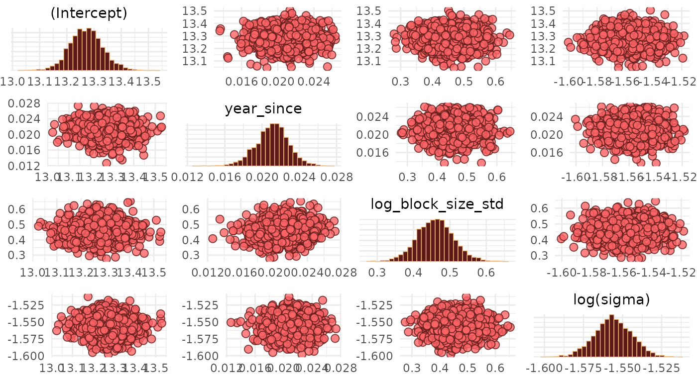

We note that there are no divergent transitions, and the Gaussian blobs/clouds suggest that there are no major issues with our estimates (see Visual MCMC diagnostics using the bayesplot package for a lot more details on MCMC diagnostics).

Next, we compare samples drawn from the posterior predictive distribution with $\mathtt{log\_UV}$ values, and show the distribution of leave-one-out (LOO)-adjusted R-squared values $R^2_s$ .

ppc_dens_overlay(data_model$log_UV, posterior_predict(model)) +
    labs(
        x = "log(UV)",
        y = "density",
        title = "Posterior predictive check")
loo_r2 <- loo_R2(model)
#> Warning: Some Pareto k diagnostic values are too high. See help('pareto-k-diagnostic') for details.
loo_r2 %>%
    enframe() %>%
    ggplot(aes(value)) +
    geom_density() + 
    theme_minimal() +
    labs(
        x = "R²",
        y = "density",
        title = "Bayesian R² distribution")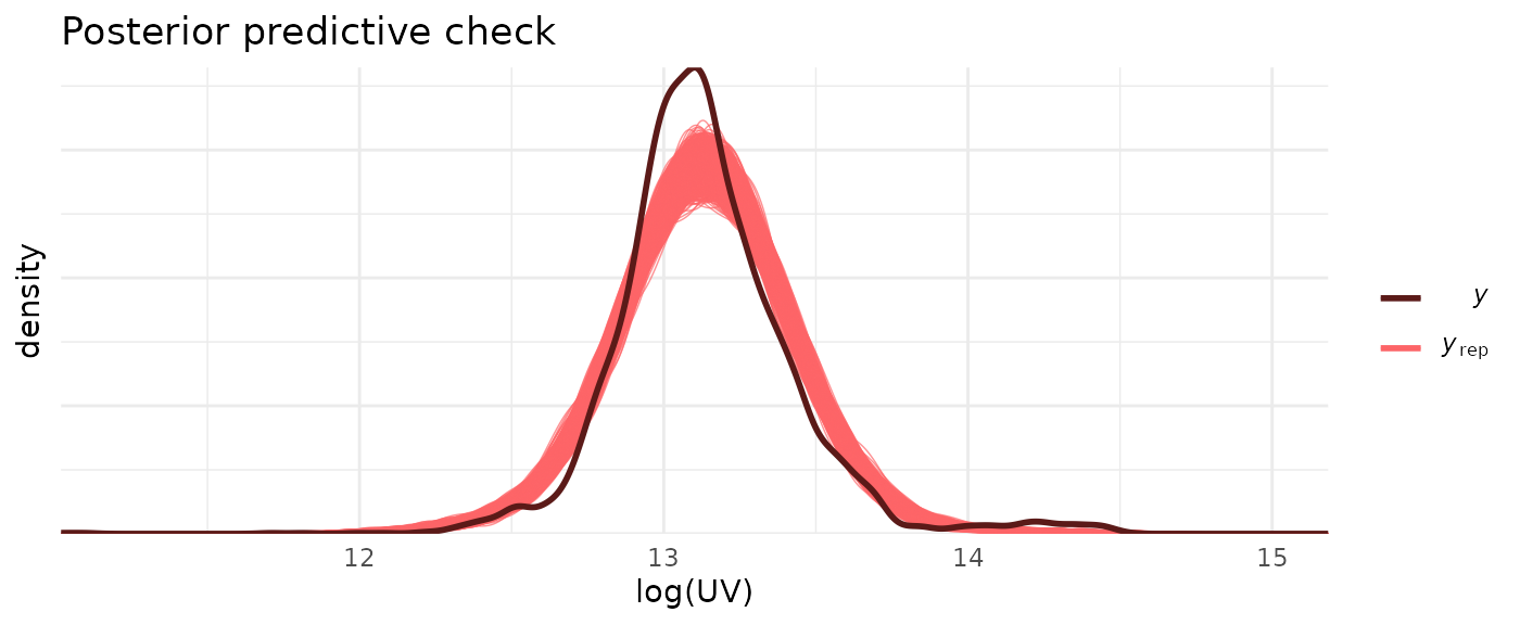

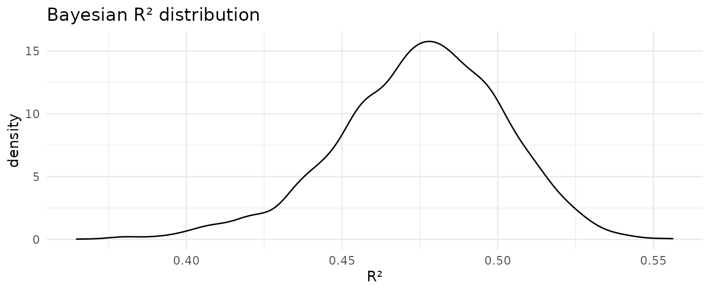
The posterior predictive check suggests some issues with the model fit. Of note, the actual $\mathtt{log\_UV}$ distribution shows a small bump at values $\log{\mathrm{UV}} > 14$ (corresponding to values greater than $1.2 million) which is not reproduced by the model. Instead these large UV values pull the mean of the posterior predictive to a slightly larger value than that of the actual distribution. The median Bayesian $R^2_s$ value of 0.53 also indicates that this is not a great fit; or in other words: there is a lot of unexplained (residual) variance.

Model results

We show and interpret fixed and random-effect parameter estimates. broom.mixed::tidy() makes it easy to extract estimates in a standardised format.

Interpretation of fixed effect estimates

We show fixed parameter estimates (mean and standard deviation) including 95% uncertainty estimates (based on the 2.5% and 97.5% quantiles of the marginal posteriors).

effect_fixed <- broom.mixed::tidy(model, "fixed", conf.int = TRUE)
effect_fixed
#> # A tibble: 3 × 5
#>   term               estimate std.error conf.low conf.high
#>   <chr>                 <dbl>     <dbl>    <dbl>     <dbl>
#> 1 (Intercept)         13.2      0.0677   13.1      13.4   
#> 2 year_since           0.0211   0.00178   0.0179    0.0243
#> 3 log_block_size_std   0.442    0.0573    0.345     0.536

The intercept estimate is $\mu_\alpha$ = 13.2. This means that the estimated fixed-effect UV in 2019 of a block the size of 850 $\mathrm{m}^2$ is approximately $\exp{(\mu_\alpha)}$ = $562.9k.
The coefficient estimate for year_since of $\mu_{\beta_1}$ = 0.0211 means that the fixed-effect UV of a block the size of 850 $\mathrm{m}^2$ increases every year by a factor of $\exp{(\mu_{\beta_1})}$ = 1.02, i.e. by around 2%.
The coefficient estimate for log_block_size_std of $\mu_{\beta_2}$ = 0.442 means that a 10% increase in block size in 2019 translated into a $\exp{(\mu_{\beta_2} \log(1.1))}$ = 1.04 factor increase in the UV, i.e. a 4% increase (in the UV).

We can compare fixed-effect estimates from the mixed-effect model with those from a complete pooling model, i.e. a model where we ignore any division-level differences.

model_complete_pooling <- stan_glm(
    log_UV ~ 1 + year_since + log_block_size_std,
    data = data_model)
broom::tidy(model_complete_pooling, "fixed", conf.int = TRUE)

We note the wider uncertainty intervals in the fixed-effect estimates of the mixed-effect model, which are probably more realistic given the variability in division-level effects.

Interpretation of random effect estimates

Random-effect estimates are shown as standard deviations of the underlying (normal) distributions and correlation coefficients of the covariance matrix. The following table summarises those estimates including the residual standard deviation $\sigma$ .

effect_random <- broom.mixed::tidy(model, "ran_pars", conf.int = TRUE)
effect_random
#> # A tibble: 7 × 3
#>   term                                        group     estimate
#>   <chr>                                       <chr>        <dbl>
#> 1 sd_(Intercept).division                     division  0.241   
#> 2 sd_year_since.division                      division  0.00457 
#> 3 sd_log_block_size_std.division              division  0.186   
#> 4 cor_(Intercept).year_since.division         division  0.158   
#> 5 cor_(Intercept).log_block_size_std.division division  0.000631
#> 6 cor_year_since.log_block_size_std.division  division -0.000164
#> 7 sd_Observation.Residual                     Residual  0.214

The standard deviation estimate for the random-effect intercept distribution of $\mathrm{sd}(\alpha_{[i]})$ = 0.241 means that 68% of properties (in 2019 with a block size of 850 $\mathrm{m}^2$ ) across all divisions have a UV in the range of $[\mu_\alpha - \mathrm{sd}(\alpha_{[i]}), \mu_\alpha + \mathrm{sd}(\alpha_{[i]})]$ = [$442.5k, $716.2k].
The standard deviation estimate for the random-effect component of the year_since effect is $\mathrm{sd}(\beta_{1,[i]})$ = 0.00457; this means that the per-year UV increase of 68% of properties (with a block size of 850 $\mathrm{m}^2$ ) across all divisions is in the range of $[\mu_{\beta_1} - \mathrm{sd}(\beta_{1,[i]}), \mu_{\beta_1} + \mathrm{sd}(\beta_{1,[i]})]$ = [1.7%, 2.6%].
The standard deviation estimate for the random-effect component of the log_block_size_std effect is $\mathrm{sd}(\beta_{2,[i]})$ = 0.186; this means that a 10% increase in block size of 68% of properties across all divisions in 2019 translated into a UV increase in the range of [2.5%, 6.2%].

Forecasts

We use the model to predict UV values across all Woden valley suburbs as a function of block size and for every 5 years between 2010 and 2030 . This is easy to do by using modelr::data_grid() to create a grid of values which are then used as input to the model; tidybayes::add_predicted_draws() then draws samples from the posterior predictive distribution conditional on the generated input data.

data_pred <- data_model %>%
    data_grid(
        division = unique(division),
        year_since = seq(2010L, 2030L, by = 5) - 2019L,
        log_block_size_std = log(seq(100, 2000, by = 10)) - log(850)) %>%
    add_predicted_draws(model) %>%
    group_by(division, year_since, log_block_size_std) %>%
    median_qi() %>%
    ungroup() %>%
    mutate(
        year = year_since + 2019L,
        block_size = exp(log_block_size_std + log(850)))

Dynamic visualisation

We now draw median and 95% quantile intervals of the UV predictions as a function of block size for every division (suburb) and year. We use plotly to produce an interactive visualisation, with details given on mouse-hover.

# Create nested data
data_pl <- data_pred %>%
    group_by(division) %>%
    nest() %>%
    ungroup()
# Silence warnings that originate from using `frame`
options(warn = -1)
# Create plotly subplots
map2(
    data_pl$division, data_pl$data,
    function(suburb, df) {
    df %>% 
        plot_ly(
            x = ~block_size, 
            frame = ~year,
            customdata = ~ sprintf(
                "<b>%s</b>, %i m²<br>Median UV: A$ %ik<br>95%% CI [%ik, %ik]<extra></extra>", 
                suburb, round(block_size),
                round(exp(.prediction) / 1e3),
                round(exp(.lower) / 1e3), round(exp(.upper) / 1e3)),
            height = 1000) %>%
        add_lines(
            y = ~exp(.prediction), 
            line = list(color = pal[1]),
            showlegend = FALSE,
            hovertemplate = "%{customdata}") %>%
        add_ribbons(
            ymin = ~exp(.lower), ymax = ~exp(.upper), 
            color = NA,
            fillcolor = pal[1],
            opacity = 0.2,
            showlegend = FALSE,
            hoverinfo = "none") %>%
        layout(
            yaxis = list(
                title = "",
                range = c(0, max(exp(df$.upper)))),
            xaxis = list(title = ""),
            annotations = list(list(
                x = 0.5, 
                y = 1, 
                text = suburb,
                xref = "paper",  
                yref = "paper",  
                xanchor = "center",  
                yanchor = "bottom",  
                showarrow = FALSE))
        ) 
    }) %>%
    subplot(
        nrows = 5, 
        shareX = TRUE) %>%
    layout(
        margin = list(t = 50, r = 10, t = 10, b = 10),
        xaxis = list(title = "Block size [m²]"),
        yaxis = list(title = "Unimproved Value (UV) [A$]")) %>%
    animation_button(visible = FALSE)

Static visualisation

We also show a static version for years 2010, 2020 and 2030, and include recorded UV data from 2020 sales.

# Reset warning level to default
options(warn = 0)
data_pred %>%
    filter(year %in% c(2010, 2020, 2030)) %>%
    mutate(year = as.factor(year)) %>%
    ggplot(aes(block_size, exp(.prediction), colour = year, fill = year)) +
    geom_point(
        data = data_model %>% filter(year == 2020L), 
        aes(x = block_size, y = unimproved_value),
        colour = pal[2],
        inherit.aes = FALSE) +
    geom_line() + 
    geom_ribbon(aes(ymin = exp(.lower), ymax = exp(.upper)), colour = NA, alpha = 0.2) +
    facet_wrap(~ division, scales = "free_y", ncol = 3) +
    scale_fill_manual(values = pal) +
    scale_colour_manual(values = pal) +
    scale_y_continuous(
        labels=scales::dollar_format(accuracy = 1, scale = 1e-3, suffix = "k")) +
    theme_minimal() +
    labs(
        x = "Block size [m²]", y = "Unimproved Value (UV) [A$]", 
        fill = "Year", colour = "Year") +
    theme(legend.position = "top")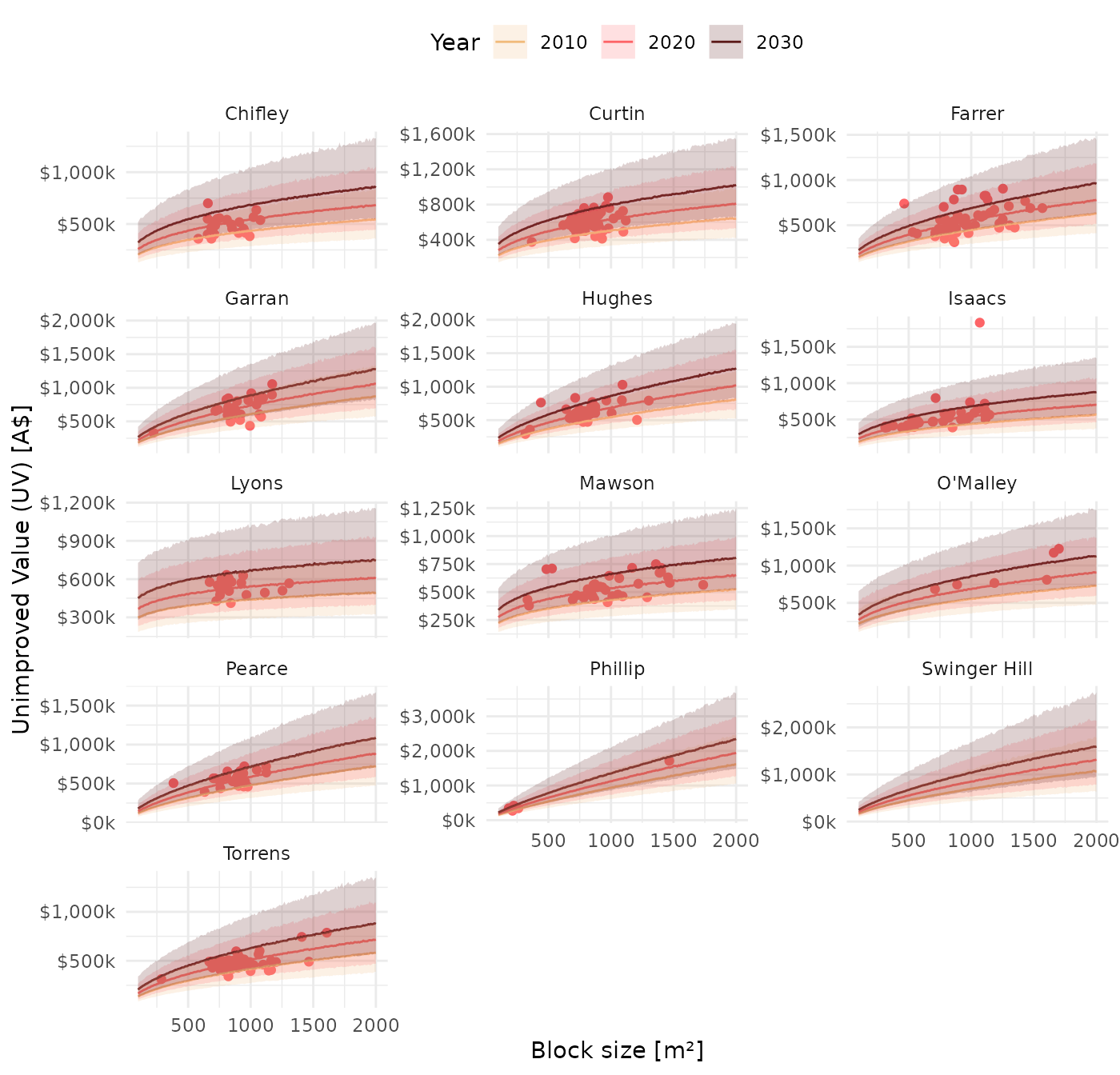

Observations

We note a few observations:

Properties of block size 1000 $m^2$ have the highest UV in the suburbs Phillip, Swinger Hill and Garran in 2030.

#> # A tibble: 3 × 6
#>   division `2010` `2015` `2020` `2025` `2030`
#>   <chr>    <chr>  <chr>  <chr>  <chr>  <chr> 
#> 1 Phillip  $950k  $1070k $1190k $1340k $1500k
#> 2 Garran   $608k  $670k  $736k  $805k  $889k 
#> 3 Hughes   $536k  $604k  $679k  $761k  $857k

Lyons, Mawson and Torrens properties of the same size are predicted to have the lowest UV om 2030.

#> # A tibble: 3 × 6
#>   division `2010` `2015` `2020` `2025` `2030`
#>   <chr>    <chr>  <chr>  <chr>  <chr>  <chr> 
#> 1 Farrer   $454k  $500k  $550k  $606k  $666k 
#> 2 Mawson   $429k  $476k  $526k  $582k  $648k 
#> 3 Torrens  $424k  $466k  $512k  $559k  $614k

The suburbs Phillip, Swinger Hill and Hughes are predicted to show the largest change in UV in 2030 relative to 2025.

#> # A tibble: 3 × 5
#>   division `2015 - 2010` `2020 - 2015` `2025 - 2020` `2030 - 2025`
#>   <chr>    <chr>         <chr>         <chr>         <chr>        
#> 1 Phillip  $116k         $127k         $145k         $157k        
#> 2 Hughes   $67.9k        $74.3k        $82.8k        $95.8k       
#> 3 Curtin   $64.6k        $73.7k        $67.9k        $84.5k

The suburbs Lyons, Mawson, and Pearce are predicted to show the smallest change in UV during that period.

#> # A tibble: 3 × 5
#>   division `2015 - 2010` `2020 - 2015` `2025 - 2020` `2030 - 2025`
#>   <chr>    <chr>         <chr>         <chr>         <chr>        
#> 1 Mawson   $46.9k        $50.2k        $56.5k        $66.1k       
#> 2 Farrer   $45.7k        $50.5k        $55.8k        $59.6k       
#> 3 Torrens  $41.7k        $46k          $46.6k        $55.5k

Maurits Evers

2026-03-21