Analysing property prices by number of bedrooms in North Canberra suburbs • allhomes

Introduction

This vignette demonstrates how to use the allhomes package to extract and analyse historical property sales data from allhomes.com.au. We’ll focus on exploring the relationship between property prices and the number of bedrooms in three northern Canberra suburbs: Watson, Ainslie, and Downer. By analysing sales data from 2018 to 2022, we’ll create visualisations to understand price distributions across different bedroom counts.

The allhomes package provides access to detailed sales data, including property features, sale prices, and dates. This example shows how to collect data for multiple suburbs and years, clean it, and perform basic exploratory data analysis.

Setup

First, load the required packages. We’ll use allhomes for Allhomes sales data extraction and tidyverse for data manipulation and visualisation.

library(allhomes)
library(tidyverse)

Data collection

The get_past_sales_data() function retrieves sales data for a specific suburb and year. We’ll collect data for three suburbs over five years (2018-2022) using a nested purrr::map_dfr approach.

# Define suburbs and years
suburbs <- c("Watson, ACT", "Ainslie, ACT", "Downer, ACT")
years <- 2018L:2022L

# Collect data using nested map_dfr
data <- suburbs |> 
    map_dfr(function(burb) 
        map_dfr(years, function(yr) 
            get_past_sales_data(burb, yr) |> 
                mutate(suburb_name = burb, sale_year = yr)))

# Check the structure of the collected data
glimpse(data)
#> Rows: 1,866
#> Columns: 24
#> $ contract_date          <date> 2018-12-17, 2018-10-18, 2018-11-12, 2018-11-02…
#> $ address                <chr> "39/215 Aspinall Street", "13/21 Aspinall Stree…
#> $ division               <chr> "Watson", "Watson", "Watson", "Watson", "Watson…
#> $ state                  <chr> "ACT", "ACT", "ACT", "ACT", "ACT", "ACT", "ACT"…
#> $ postcode               <chr> "2602", "2602", "2602", "2602", "2602", "2602",…
#> $ url                    <chr> "https://www.allhomes.com.au/unit-39-215-aspina…
#> $ property_type          <chr> "TOWNHOUSE", NA, NA, NA, "APARTMENT", NA, "UNIT…
#> $ purpose                <chr> NA, "MULTIPLE UNIT DWELLING", "SINGLE RESIDENTI…
#> $ bedrooms               <int> 3, NA, NA, NA, 2, NA, 1, 2, 3, 3, 4, 3, 4, 4, 3…
#> $ bathrooms              <int> 2, NA, NA, NA, 2, NA, 1, 2, 2, 2, 3, 1, 2, 2, 2…
#> $ parking                <int> 2, NA, NA, NA, 2, NA, 0, 2, 2, 2, 2, 2, 2, 2, 2…
#> $ building_size          <int> NA, NA, NA, NA, NA, NA, NA, 0, NA, NA, 0, NA, 2…
#> $ block_size             <int> NA, 17228, 680, 2302, 20536, 830, 4365, 20536, …
#> $ eer                    <dbl> 3.0, NA, NA, NA, 5.0, NA, 5.0, 4.0, 3.0, 3.0, 6…
#> $ list_date              <date> 2018-11-28, NA, NA, NA, 2018-08-22, NA, 2018-1…
#> $ transfer_date          <date> NA, 2018-12-17, 2018-12-17, 2018-12-17, 2018-1…
#> $ days_on_market         <int> 19, NA, NA, NA, 82, NA, 29, 43, 34, 155, 23, 23…
#> $ label                  <chr> "Sold", "Sold", "Sold", "Sold", "Sold", "Sold",…
#> $ price                  <int> 595000, 516000, 715000, 368000, 360000, 760000,…
#> $ agent                  <chr> "Independent Gungahlin", NA, NA, NA, "Sadil Qui…
#> $ unimproved_value       <int> NA, NA, NA, NA, NA, NA, NA, NA, NA, 567000, 557…
#> $ unimproved_value_ratio <dbl> NA, NA, NA, NA, NA, NA, NA, NA, NA, 0.7105263, …
#> $ suburb_name            <chr> "Watson, ACT", "Watson, ACT", "Watson, ACT", "W…
#> $ sale_year              <int> 2018, 2018, 2018, 2018, 2018, 2018, 2018, 2018,…

Data exploration

Let’s examine the collected data. We’ll look at the total number of sales, data completeness, and basic statistics.

# Summary statistics
data %>%
    group_by(suburb_name, sale_year) |>
    summarise(
        total_sales = n(),
        sales_with_bedrooms = sum(!is.na(bedrooms) & bedrooms > 0),
        sales_with_price = sum(!is.na(price) & price > 0),
        median_price = median(price, na.rm = TRUE),
        .groups = "drop") |>
    knitr::kable(caption = "Summary of sales data by suburb and year")

Summary of sales data by suburb and year
suburb_name	sale_year	total_sales	sales_with_bedrooms	sales_with_price	median_price
Ainslie, ACT	2018	68	44	67	1067500
Ainslie, ACT	2019	72	37	70	900000
Ainslie, ACT	2020	64	35	64	1170000
Ainslie, ACT	2021	88	32	88	1325000
Ainslie, ACT	2022	65	25	64	1570000
Downer, ACT	2018	73	51	73	793000
Downer, ACT	2019	68	44	68	795000
Downer, ACT	2020	71	45	71	800000
Downer, ACT	2021	126	34	126	709900
Downer, ACT	2022	87	49	86	1238000
Watson, ACT	2018	149	121	149	520000
Watson, ACT	2019	162	117	162	613000
Watson, ACT	2020	265	108	265	530000
Watson, ACT	2021	273	112	273	570000
Watson, ACT	2022	235	97	234	600000

Price analysis by bedrooms

Now we’ll analyse how property prices vary with the number of bedrooms. We’ll filter for valid data and create a boxplot to visualise price distributions.

# Filter and prepare data for plotting
plot_data <- data |>
    filter(
        !is.na(bedrooms), bedrooms > 0, bedrooms <= 6, # Reasonable bedroom range
         !is.na(price), price > 0, price < 10e6)       # Reasonable price range

# Create boxplot
plot_data |>
    ggplot(aes(x = as.factor(bedrooms), y = price)) +
    geom_boxplot() +
    scale_y_continuous(
        labels = scales::label_dollar(scale = 1e-6, suffix = "M")) +
    facet_wrap(~ suburb_name) +
    labs(
        title = "Property sale prices by number of bedrooms",
        subtitle = "Data from Watson, Ainslie, and Downer (ACT); 2018-2022",
        x = "Number of bedrooms",
        y = "Sale price (AUD)") +
    theme_minimal()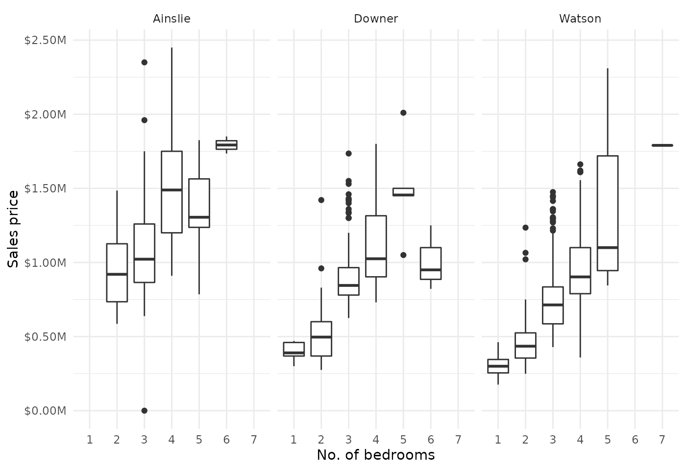

Insights

From the visualisation, we can observe:

Price trends: Generally & unsurprisingly, properties with more bedrooms result in higher sale prices, though there exists significant variation within each category.
Suburb differences: Price distributions vary between suburbs, reflecting local market conditions.
Data considerations: Not all sales records include bedroom information, and some outliers may affect the distributions.

This analysis provides a starting point for deeper exploration. Potential extensions could include:

Analysing price per bedroom
Examining trends over time
Including additional property features like bathrooms or land size