Median sale prices across Sydney Leichhardt suburbs in 2021
Introduction
This vignette demonstrates how to use the allhomes package to extract and analyse historical property sales data from allhomes.com.au. We’ll focus on exploring median property sale prices across suburbs in the Sydney Leichhardt area during 2021. By analysing sales data from multiple suburbs, we’ll create visualisations to understand price distributions and identify patterns in the local property market.
The allhomes package provides access to detailed sales data, including property features, sale prices, and dates. This example shows how to collect data for multiple suburbs, clean it, and perform basic exploratory data analysis to understand median price variations.
Setup
First, load the required packages. We’ll use allhomes for Allhomes sales data extraction, tidyverse for data manipulation and visualisation, and ggbeeswarm for creating bee swarm plots.
Data collection
The get_past_sales_data() function retrieves sales data for a specific suburb and year. We’ll collect data for all suburbs in the Leichhardt SA3 area using the internal divisions_NSW dataset to identify the relevant suburbs.
# Get all Leichhardt suburbs
suburbs <- divisions_NSW |>
    filter(sa3_name_2016 == "Leichhardt") |>
    unite(suburb, division, state, sep = ", ") |>
    pull(suburb)

# Display the suburbs we're analysing
suburbs
#> [1] "Annandale, NSW"    "Balmain, NSW"      "Balmain East, NSW"
#> [4] "Birchgrove, NSW"   "Leichhardt, NSW"   "Lilyfield, NSW"
#> [7] "Rozelle, NSW"

# Get data for Leichhardt suburbs
data <- suburbs |> map(get_past_sales_data, year = 2021L) |> bind_rows()
Data exploration
Let’s examine the collected data. We’ll look at the total number of sales, data completeness, and basic statistics by suburb and property type.
# Summary statistics by suburb and property type
data_summary <- data %>%
    group_by(division, property_type) |>
    summarise(
        total_sales = n(),
        sales_with_price = sum(!is.na(price) & price > 0),
        median_price = median(price, na.rm = TRUE),
        mean_price = mean(price, na.rm = TRUE),
        .groups = "drop") |>
    arrange(division, property_type)

# Display summary table
data_summary |>
    knitr::kable(
        caption = "Summary of sales data by suburb and property type (2021)",
        digits = 0,
format.args = list(big.mark = ","))| division | property_type | total_sales | sales_with_price | median_price | mean_price |
|---|---|---|---|---|---|
| Annandale | APARTMENT | 30 | 2 | 1,180,000 | 1,180,000 |
| Annandale | HOUSE | 108 | 14 | 1,787,500 | 2,185,000 |
| Annandale | TOWNHOUSE | 11 | 2 | 1,862,500 | 1,862,500 |
| Annandale | UNIT | 1 | 1 | 500,000 | 500,000 |
| Annandale | NA | 77 | 52 | 1,190,000 | 1,157,981 |
| Balmain | APARTMENT | 48 | 7 | 860,000 | 833,643 |
| Balmain | HOUSE | 126 | 22 | 2,056,000 | 2,738,455 |
| Balmain | TOWNHOUSE | 7 | 1 | 1,396,000 | 1,396,000 |
| Balmain | NA | 82 | 63 | 1,662,500 | 1,788,098 |
| Balmain East | APARTMENT | 8 | 2 | 1,270,000 | 1,270,000 |
| Balmain East | HOUSE | 14 | 1 | 2,700,000 | 2,700,000 |
| Balmain East | TOWNHOUSE | 2 | 0 | NA | NaN |
| Balmain East | NA | 16 | 10 | 1,743,500 | 2,009,188 |
| Birchgrove | APARTMENT | 11 | 1 | 1,030,000 | 1,030,000 |
| Birchgrove | HOUSE | 40 | 2 | 3,800,000 | 3,800,000 |
| Birchgrove | TOWNHOUSE | 5 | 1 | 2,000,000 | 2,000,000 |
| Birchgrove | NA | 21 | 13 | 1,750,000 | 1,900,952 |
| Leichhardt | APARTMENT | 55 | 5 | 725,000 | 820,000 |
| Leichhardt | HOUSE | 171 | 16 | 1,505,000 | 1,582,156 |
| Leichhardt | LAND | 1 | 0 | NA | NaN |
| Leichhardt | TOWNHOUSE | 26 | 2 | 1,100,000 | 1,100,000 |
| Leichhardt | NA | 107 | 79 | 1,265,000 | 1,103,242 |
| Lilyfield | APARTMENT | 12 | 2 | 857,500 | 857,500 |
| Lilyfield | HOUSE | 85 | 10 | 1,787,500 | 2,048,000 |
| Lilyfield | TOWNHOUSE | 6 | 1 | 979,000 | 979,000 |
| Lilyfield | NA | 64 | 42 | 1,475,000 | 1,206,052 |
| Rozelle | APARTMENT | 48 | 9 | 1,395,000 | 1,545,667 |
| Rozelle | HOUSE | 110 | 15 | 1,626,000 | 1,783,200 |
| Rozelle | TOWNHOUSE | 8 | 1 | 1,330,000 | 1,330,000 |
| Rozelle | NA | 78 | 60 | 1,314,250 | 1,255,769 |
Median price analysis
Now we’ll analyse the median sale prices across Leichhardt suburbs. We’ll filter for valid data and create a visualisation showing price distributions and median values for different property types.
# Prepare data for plotting
plot_data <- data |>
    filter(!is.na(price), price > 1e3) |>  # Remove invalid prices
    mutate(median_price = median(price), .by = property_type)  # Calculate median per property type

# Create bee swarm plot with median lines
plot_data |>
    ggplot(aes(division, price, colour = property_type)) +
    geom_quasirandom(dodge.width = 0.8, alpha = 0.7) +
    geom_errorbar(
        aes(ymin = median_price, ymax = median_price),
        position = position_dodge(width = 0.8),
        linewidth = 1) +
    scale_y_continuous(
        labels = scales::label_dollar(scale = 1e-6, suffix = "M")) +
    labs(
        title = "Property sale prices across Leichhardt suburbs (2021)",
        subtitle = "Bee swarm plot showing individual sales with median price lines",
        x = "Leichhardt suburb",
        y = "Sales price (AUD)",
        colour = "Property type") +
    theme_minimal()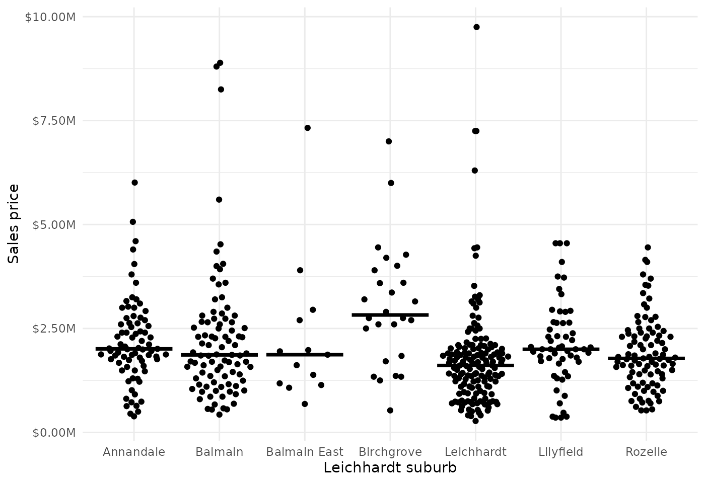
Insights
From the visualisation and data analysis, we can observe:
- Price variation by suburb: There are clear differences in median property prices between suburbs within the Leichhardt area, reflecting local market conditions and property characteristics.
- Property type differences: As expected, different property types (houses, units, etc.) show distinct price distributions, with houses generally resulting in higher prices.
- Data considerations: The bee swarm plot reveals the distribution of individual sales, while the horizontal lines show median prices for each property type across all suburbs.
This analysis provides a foundation for understanding the Leichhardt property market in 2021. Potential extensions could include:
- Analysing price trends over multiple years
- Examining the relationship between price and property features (bedrooms, bathrooms, land size)
- Investigating seasonal patterns in sales
- Comparing Leichhardt prices with other Sydney areas